Quickstart

First ensure you have installed Python 3.7 (or greater) and ELFI. After installation you can start using ELFI:

import elfi

ELFI includes an easy to use generative modeling syntax, where the generative model is specified as a directed acyclic graph (DAG). Let’s create two prior nodes:

mu = elfi.Prior('uniform', -2, 4)
sigma = elfi.Prior('uniform', 1, 4)

The above would create two prior nodes, a uniform distribution from -2 to 2 for the mean mu and another uniform distribution from 1 to 5 for the standard deviation sigma. All distributions from scipy.stats are available.

For likelihood-free models we typically need to define a simulator and summary statistics for the data. As an example, lets define the simulator as 30 draws from a Gaussian distribution with a given mean and standard deviation. Let’s use mean and variance as our summaries:

import scipy.stats as ss
import numpy as np

def simulator(mu, sigma, batch_size=1, random_state=None):
    mu, sigma = np.atleast_1d(mu, sigma)
    return ss.norm.rvs(mu[:, None], sigma[:, None], size=(batch_size, 30), random_state=random_state)

def mean(y):
    return np.mean(y, axis=1)

def var(y):
    return np.var(y, axis=1)

Let’s now assume we have some observed data y0 (here we just create some with the simulator):

# Set the generating parameters that we will try to infer
mean0 = 1
std0 = 3

# Generate some data (using a fixed seed here)
np.random.seed(20170525)
y0 = simulator(mean0, std0)
print(y0)

[[ 3.7990926   1.49411834  0.90999905  2.46088006 -0.10696721  0.80490023
   0.7413415  -5.07258261  0.89397268  3.55462229  0.45888389 -3.31930036
  -0.55378741  3.00865492  1.59394854 -3.37065996  5.03883749 -2.73279084
   6.10128027  5.09388631  1.90079255 -1.7161259   3.86821266  0.4963219
   1.64594033 -2.51620566 -0.83601666  2.68225112  2.75598375 -6.02538356]]

Now we have all the components needed. Let’s complete our model by adding the simulator, the observed data, summaries and a distance to our model:

# Add the simulator node and observed data to the model
sim = elfi.Simulator(simulator, mu, sigma, observed=y0)

# Add summary statistics to the model
S1 = elfi.Summary(mean, sim)
S2 = elfi.Summary(var, sim)

# Specify distance as euclidean between summary vectors (S1, S2) from simulated and
# observed data
d = elfi.Distance('euclidean', S1, S2)

If you have graphviz installed to your system, you can also visualize the model:

# Plot the complete model (requires graphviz)
elfi.draw(d)

Note

The automatic naming of nodes may not work in all environments e.g. in interactive Python shells. You can alternatively provide a name argument for the nodes, e.g. S1 = elfi.Summary(mean, sim, name='S1').

We can try to infer the true generating parameters mean0 and std0 above with any of ELFI’s inference methods. Let’s use ABC Rejection sampling and sample 1000 samples from the approximate posterior using threshold value 0.5:

rej = elfi.Rejection(d, batch_size=10000, seed=30052017)
res = rej.sample(1000, threshold=.5)
print(res)

Method: Rejection
Number of samples: 1000
Number of simulations: 120000
Threshold: 0.492
Sample means: mu: 0.748, sigma: 3.1

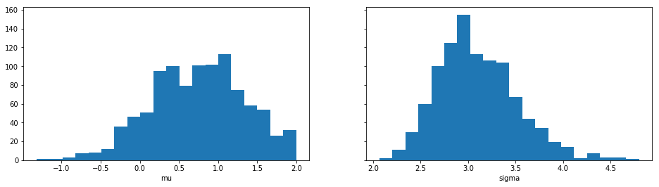
Let’s plot also the marginal distributions for the parameters:

import matplotlib.pyplot as plt
res.plot_marginals()
plt.show()